Lecture 7: Gambler's Ruin and Random Variables | Statistics 110
Harvard University・2 minutes read
The course focuses on conditional probability and random variables, pivotal concepts for the entire semester, with a particular emphasis on "Gambler's Ruin" problem and difference equations. Random variables are introduced to simplify notation and represent changing quantities in mathematical problems, with the Bernoulli and Binomial distributions playing a crucial role in calculating probabilities for different outcomes.
Insights
- Understanding conditional probability and random variables is foundational to statistics, with a focus on conditioning crucial for grasping the subject's essence.
- Difference equations, often overshadowed by their differential counterparts, offer a realistic approach for discrete observations over time, with solutions derived through root finding and linear combinations, providing valuable insights into scenarios like the "Gambler's Ruin" problem and random walk applications.
Get key ideas from YouTube videos. It’s free
Recent questions
What is conditional probability?
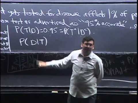
The concept of conditional probability is a key topic in statistics that involves calculating the likelihood of an event occurring given that another event has already occurred. It is crucial for understanding the relationship between events and their outcomes.
What is the "Gambler's Ruin" problem?
The "Gambler's Ruin" problem involves two players betting dollars back and forth until one player goes bankrupt, leaving the other with all the money. The goal is to determine the probability of one player winning the entire game, which has applications in various fields like finance and physics.
How are difference equations important?
Difference equations are crucial for modeling observations over time, especially when observations are discrete. They are often neglected in teaching despite being as important as differential equations. Difference equations provide a more realistic approach to understanding changing quantities over time.
What are random variables?
Random variables are introduced to simplify notation and represent changing quantities in mathematical problems. They are defined as functions from the sample space to the real line, capturing the randomness in experiment outcomes. Random variables play a significant role in probability theory and statistics.
What is the Binomial distribution?
The Binomial distribution describes the number of successes in N independent Bernoulli trials, where each trial has two possible outcomes with specified probabilities. It is used to calculate the probabilities associated with different outcomes in a series of trials. The distribution is fundamental in probability theory and statistics.
Related videos
Harvard University
Lecture 4: Conditional Probability | Statistics 110

Gresham College
Lottery-Winning Maths
Harvard University
Lecture 5: Conditioning Continued, Law of Total Probability | Statistics 110
Harvard University
Lecture 8: Random Variables and Their Distributions | Statistics 110

JEE Nexus by Unacademy
Binomial Theorem Class 11 | One Shot | JEE Main & Advanced | Arvind Kalia Sir


Summary
00:00
"Conditional Probability and Random Variables Explained"
- Conditional probability is a key topic for the semester, along with random variables and their distributions.
- The essence of statistics lies in conditioning, crucial for understanding the subject.
- The course focuses on conditioning and random variables, pivotal concepts for the entire semester.
- The instructor draws inspiration from a TV show's segment where guests explain complex topics in five words or less.
- The class will delve into random variables after discussing conditional probability.
- The "Gambler's Ruin" problem involves two players betting dollars back and forth until one goes bankrupt.
- The game ends when one player goes bankrupt, leaving the other with all the money.
- The problem aims to determine the probability of one player winning the entire game.
- The setup involves two gamblers exchanging dollars in a series of independent bets.
- The problem is akin to a random walk scenario, crucial for various applications in finance and physics.
16:16
Neglected Importance of Difference Equations in Teaching
- Difference equations are considered as important as differential equations but are often neglected in teaching.
- The speaker found it frustrating that a Google search for difference equations led to results on differential equations.
- Difference equations are more realistic for observations over time, as observations are typically discrete.
- The speaker aims to solve a specific difference equation in a different way than traditional methods.
- Guessing a solution form of x to the I is a common method for solving differential equations.
- The quadratic equation derived from the guess simplifies to 2p - 1^2ar, making the solution straightforward.
- The general solution for difference equations involves finding roots and creating a linear combination of those roots.
- The explicit solution for the specific difference equation is pi equals 1 - Q over P to the I over 1 - Q over P to the n.
- If P equals Q, the game is fair, and the solution simplifies to I over n.
- Numerical calculations show that in an unfair game, the probability of winning decreases as the game progresses, leading to the gambler's ruin.
32:09
Probability and Random Variables in Mathematics
- In the fair case, adding I over n plus n minus I over n equals one, indicating the probability of A winning and B going bankrupt.
- This probability ensures that the game does not continue indefinitely, with a probability of zero for the game to go on forever.
- The sum of the probabilities of A and B winning equals one, indicating no leftover probability for the game to continue.
- Random variables are introduced to simplify notation and represent changing quantities in mathematical problems.
- The definition of a random variable as a function from the sample space to the real line is crucial.
- Randomness in random variables stems from the randomness in the experiment's outcomes.
- The Bernoulli distribution involves a random variable with two possible values, zero and one, based on probabilities.
- The Binomial distribution describes the number of successes in N independent Bernoulli trials, with probabilities specified for different outcomes.
- The distribution of a random variable outlines the probabilities associated with its different possible values.
- Calculating probabilities for random variables like the number of successes in trials is straightforward and relies on understanding the outcomes and probabilities involved.
48:49
Calculating Success Probability in Binomial Trials
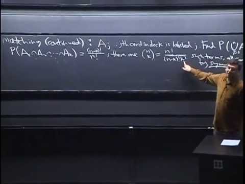
- The probability of having K successes in N trials can be calculated using the formula P^K * (1 - P)^(N-K), where P represents success and 1-P represents failure. This is known as the probability mass function (pmf) and is denoted as n choose K * P^K.
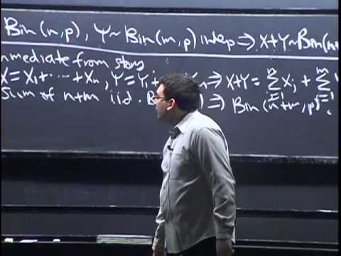
- If X is binomial NP and Y is also binomial NP, and they are independent, then X + Y will be binomial N+M P, where N and M represent the number of trials for X and Y respectively. This can be intuitively understood as the total number of successes from both X and Y trials.